Species distributions, marine heatwaves and trawling in northern Spain (GSA 6) and the Adriatic (GSAs 17-18). Working group report, Global Fishing Watch Mediterranean Data Lab
climate-env-ais working group
2026-11-03
Overview
This report brings together the four exercises of the working group into one reproducible document. The question running through all of them is how climate and environmental conditions relate to the distribution of demersal fish and to the behaviour of the trawl fleet, as seen through AIS.
Table 1: Analysis steps of this report. Step: report section. Script: the group’s R script that runs the step, or where the step is done. Question: what the step asks. Main output: files the step writes (in data/processed/ or outputs/, unless marked as group files).
Step
Script
Question
Main output
1
scripts/1_data exploration.R
What do the survey, environmental and AIS data look like, and how do they join?
data/processed/MEDITS_and_environment.csv
2a
scripts/2_SDMs.R
How does total fish abundance relate to the environment, and how has habitat suitability changed 2012-2021?
Which areas combine heatwave exposure, habitat loss and fishing pressure?
outputs/CFVI_GSA6.csv
Steps the group already ran that call the Global Fishing Watch API, read the large prediction grid or need the daily SST NetCDF are shown but not re-run (marked not evaluated). Their saved outputs are loaded instead. Everything else runs when the report is rendered, including the red mullet model of Section 2b, which is new.
The study area is GSA 6 (northern Spain), the GFCM Geographical Sub-Area covering the Spanish Mediterranean coast from Murcia to the French border, and the fleet is restricted to trawlers, the gear sampled by MEDITS.
1. Data preparation
1.1 Data sources
MEDITS (Mediterranean International Trawl Survey), 2012-2021, from the JRC data portal: abundance (N/km²) and biomass (kg/km²) per species and haul. MEDITS is a standardised bottom-trawl survey run every year, mostly in late spring and early summer.
Environmental variables at each haul, from the Copernicus Marine Mediterranean physics (MEDSEA_MULTIYEAR_PHY_006_004) and biogeochemistry (MEDSEA_MULTIYEAR_BGC_006_008) reanalyses: sea surface and bottom temperature (sst, botTemp), surface and bottom salinity (so, botso), chlorophyll (chl) and primary production (nppv), plus substrate and depth.
AIS apparent fishing hours from Global Fishing Watch, trawlers only, yearly, 0.1° cells, GFCM area, pulled with gfwr::gfw_ais_fishing_hours().
Load MEDITS and pull yearly trawler effort with gfwr (not evaluated)
Discussion point: grid alignment. GFW returns the lower-left corner of each cell, while the haul coordinates are rounded to the nearest 0.1°. Roughly half the hauls are therefore matched to a neighbouring cell. Flooring the haul coordinates (floor(x * 10) / 10) would align the two.
1.2 The merged dataset
Load the merged survey, environment and effort table
med <-read.csv("data/processed/MEDITS_and_environment.csv")hauls <-distinct(med, id, .keep_all =TRUE)
The merged table holds 427,911 species-by-haul records from 12,368 hauls across 18 GSAs.
Interactive map of MEDITS hauls (R/haul_map.R, shared with the slides)
source("R/haul_map.R")hauls_map <- hauls |>transmute(id, GSA, country = COUNTRY, year = YEAR, month = MONTH,lon = MEAN_LONGITUDE_DEC, lat = MEAN_LATITUDE_DEC,depth = MEAN_DEPTH, sst, botTemp, fishing_hours)saveRDS(hauls_map, "outputs/hauls_map.rds") # read by the slideshaul_map(hauls_map, height =520)
MEDITS hauls 2012-2021, coloured by GSA on a dark-blue background, with GSA 6 in gold. Hover over a haul for its date, depth, bottom temperature, SST and the AIS trawling effort in its grid cell; drag to pan and scroll to zoom.
Show code
hpy <- hauls |>count(GSA, YEAR) |>complete(GSA, YEAR =2012:2021) |># explicit NA so missing years break the linemutate(GSA =factor(GSA))ends <- hpy |>filter(!is.na(n)) |>group_by(GSA) |>slice_max(YEAR, n =1)cols <-gsa_colours(hauls$GSA)cols["6"] <-"#d9a520"# GSA 6 in gold, as on the mapggplot(hpy, aes(YEAR, n, colour = GSA, group = GSA)) +geom_line(aes(linewidth = GSA =="6"), na.rm =TRUE) +geom_point(size =1.4, na.rm =TRUE) + ggrepel::geom_text_repel(data = ends, aes(label =paste("GSA", GSA)),nudge_x =0.35, direction ="y", hjust =0, size =3.3,segment.colour ="grey70", segment.size =0.3,min.segment.length =0, box.padding =0.12, seed =1) +scale_colour_manual(values = cols, guide ="none") +scale_linewidth_manual(values =c(`FALSE`=0.6, `TRUE`=1.6), guide ="none") +scale_x_continuous(breaks =2012:2021, expand =expansion(mult =c(0.02, 0.16))) +labs(x =NULL, y ="Hauls per year") +theme_ocean() +theme(panel.grid.major.x =element_blank())
Figure 1: Number of MEDITS hauls per year in each GSA (colours as in the map; GSA 6 in bold gold). Breaks in a line, and isolated points, are years without a survey in that GSA.
Most GSAs are sampled at a near-constant number of hauls each year, but there are three notable exceptions: 2020 is missing in GSAs 1, 2 and 8 and roughly halved in GSAs 6, 7 and 10, most likely because of COVID-19 restrictions; the Greek GSAs (20, 22, 23) were not surveyed every year before 2018; and GSA 17 roughly doubled its sampling from 2013. In GSA 6, 2020 has 52 hauls against about 100 in other years, which matters for any year-by-year comparison.
Figure 2: Sea surface temperature at the time of each haul.
1.3 What AIS sees over time
Before using AIS effort as a covariate, it is worth checking how its coverage changes over the study period.
Show code
ais_cov <- hauls |>group_by(YEAR) |>summarise(matched =mean(!is.na(fishing_hours)),mean_hours =mean(fishing_hours, na.rm =TRUE), .groups ="drop")(ggplot(ais_cov, aes(YEAR, matched)) +geom_col(fill = pal_ocean[["surface"]]) +scale_y_continuous(labels = percent) +labs(title ="Hauls with AIS effort", x =NULL, y =NULL)) +(ggplot(ais_cov, aes(YEAR, mean_hours)) +geom_line(colour = pal_ocean[["deep"]]) +geom_point(colour = pal_ocean[["deep"]]) +labs(title ="Mean trawler hours per matched haul cell", x =NULL, y =NULL)) &scale_x_continuous(breaks =2012:2021) &theme_ocean()
Figure 3: Share of MEDITS hauls with matched AIS trawler effort, and mean effort at matched hauls, by year. The 2012-2014 increase reflects AIS adoption by the fleet rather than more fishing.
In 2012, only 49% of hauls fall in a cell with any AIS trawler effort, against 98% in 2021. Mean effort at matched hauls rises from 64 hours in 2012 to 835 in 2015, then stabilises.
Discussion point: AIS ramp-up. Trawler AIS coverage at MEDITS hauls grows sharply over 2012-2014. Any comparison across these years (habitat change in Step 2, heatwave vs non-heatwave summers in Step 3) partly measures AIS uptake. Options: start in 2015, use effort per vessel, or treat early years separately.
2. Species distribution models
Three species distribution models (SDMs) relate MEDITS survey catches to the environment and to trawling effort, and predict them on the Copernicus grid. Section 2a models total fish abundance in GSA 6 with the group’s original script; Section 2b applies the same workflow to red mullet (Mullus barbatus), the group’s focal species; Section 2c presents the group’s spatio-temporal model of red mullet in GSA 6 and the Adriatic (GSAs 17-18), and builds on it to relate red mullet to marine heatwaves and trawling.
2a. Species distribution model: total fish abundance
2a.1 Response variable
Species distribution models (SDMs) relate biological observations to environmental conditions to estimate habitat suitability and predict into unsampled locations. Here the response is total fish abundance per haul (N/km², all MEDITS faunistic categories A, Aa, Ae, Ao), modelled within a single GSA so that species-habitat relationships are reasonably homogeneous.
Figure 5: Pairwise Pearson correlations among candidate predictors in GSA 6 hauls. Variables are ordered by hierarchical clustering so that correlated groups sit together; pairs with |r| above 0.6 are outlined.
The group’s script uses usdm::vif() and vifstep(th = 3). The same variance inflation factors are computed below from auxiliary regressions.
Table 2: Variance inflation factors (VIF) of the candidate predictors of the total fish model, GSA 6 hauls. variable: predictor (sst: sea surface temperature, °C; botTemp: bottom temperature, °C; so: surface salinity, PSU; botso: bottom salinity, PSU; chl: surface chlorophyll-a, mg/m³; MEAN_DEPTH: mean haul depth, m; fishing_hours: GFW AIS apparent trawler fishing hours in the haul’s 0.1° cell and year). VIF: 1 / (1 − R²) of the regression of that predictor on all the others; values above 3 indicate problematic collinearity.
variable
VIF
sst
1.30
botTemp
2.43
so
1.10
botso
3.14
chl
1.53
MEAN_DEPTH
2.85
fishing_hours
1.16
Collinearity is moderate overall. Bottom salinity (botso) is the only variable above the VIF threshold of 3, driven by its correlation with depth (r = 0.79) and bottom temperature (r = -0.63), and is dropped. Depth (VIF just under 3) is left out of the candidate set, its information being largely carried by bottom temperature.
2a.3 GAM fitting and selection
Generalised additive models (GAMs, mgcv) allow smooth, non-linear responses. Smooths are capped at k = 4 to keep response curves ecologically interpretable, and select = TRUE adds a shrinkage penalty so that unhelpful terms can be shrunk to zero. Hauls with any missing predictor are removed.
Fit the full and reduced GAMs
fish6 <-na.omit(fish6)gam1 <-gam(log_N_km2 ~s(sst, k =4) +s(botTemp, k =4) +s(so, k =4) +s(chl, k =4) +s(fishing_hours, k =4),family = gaussian, data = fish6, method ="REML", select =TRUE)gam2 <-gam(log_N_km2 ~s(botTemp, k =4) +s(so, k =4) +s(chl, k =4) +s(fishing_hours, k =4),family = gaussian, data = fish6, method ="REML", select =TRUE)gam_tab <-tibble(model =c("gam1: full", "gam2: without SST"),n =c(nobs(gam1), nobs(gam2)),`R² (adj.)`=round(c(summary(gam1)$r.sq, summary(gam2)$r.sq), 3),`Deviance explained`=percent(c(summary(gam1)$dev.expl, summary(gam2)$dev.expl), 0.1),AIC =round(c(AIC(gam1), AIC(gam2)), 1))
Table 3: Comparison of the two total fish GAMs (Gaussian, response log(N/km²)). model: predictor set (gam1: bottom temperature, SST, surface salinity, chlorophyll and fishing hours; gam2: the same without SST). n: number of hauls used. R² (adj.): adjusted R². Deviance explained: share of the null deviance explained by the model. AIC: Akaike information criterion (lower is better).
Table 4: Smooth terms of the retained total fish model (gam2). term: smooth function s() of each predictor. edf: effective degrees of freedom (1 = linear; close to 0 = shrunk out of the model by select = TRUE). F: test statistic for the term. p-value: approximate significance of the term.
Table 5: Six best models of the all-subsets selection on gam1 (MuMIn::dredge), ranked by AICc. s() columns: ‘+’ if the smooth of that predictor is in the model, blank if not. df: number of estimated parameters. logLik: log-likelihood. AICc: AIC corrected for small samples. delta: AICc difference from the best model. weight: Akaike weight, the relative support for each model among all those fitted.
s(botTemp, k = 4)
s(chl, k = 4)
s(fishing_hours, k = 4)
s(so, k = 4)
s(sst, k = 4)
df
logLik
AICc
delta
weight
16
+
+
+
+
9
-1490.88
3000.98
0.00
0.32
32
+
+
+
+
+
9
-1490.88
3000.99
0.00
0.32
12
+
+
+
7
-1493.40
3002.61
1.62
0.14
28
+
+
+
+
7
-1493.40
3002.61
1.62
0.14
14
+
+
+
8
-1494.05
3005.35
4.36
0.04
30
+
+
+
+
9
-1492.70
3005.48
4.49
0.03
Show code
# ggplot partial-effect plots for an mgcv GAM (no extra packages needed)gam_smooths <-function(model, residuals =TRUE, ncol =2, n =200) { dat <- model$model resp <-all.vars(formula(model))[1] st <-summary(model)$s.table med <-lapply(dat[setdiff(names(dat), resp)], \(x) if (is.numeric(x)) median(x, na.rm =TRUE) else x[1]) term_obs <-predict(model, type ="terms") res_w <-residuals(model, type ="working") pieces <-lapply(model$smooth, function(sm) { v <- sm$term lab <- sm$label head <-sprintf("%s · edf %.2f, p %s", unname(var_labels[v]) %||% v, st[lab, "edf"],format.pval(st[lab, 4], digits =2, eps =1e-4)) nd <-as.data.frame(med)[rep(1, n), , drop =FALSE] nd[[v]] <-seq(min(dat[[v]]), max(dat[[v]]), length.out = n) p <-predict(model, nd, type ="terms", se.fit =TRUE)list(curve =tibble(term = head, x = nd[[v]], fit = p$fit[, lab],lo = p$fit[, lab] -1.96* p$se.fit[, lab],hi = p$fit[, lab] +1.96* p$se.fit[, lab]),pts =tibble(term = head, x = dat[[v]], pr = term_obs[, lab] + res_w)) }) curves <-bind_rows(lapply(pieces, `[[`, "curve")) pts <-bind_rows(lapply(pieces, `[[`, "pts")) lvls <-unique(curves$term) curves$term <-factor(curves$term, lvls); pts$term <-factor(pts$term, lvls) g <-ggplot(curves, aes(x)) +geom_hline(yintercept =0, colour ="grey75", linewidth =0.4)if (residuals) g <- g +geom_point(data = pts, aes(x, pr), colour = pal_ocean[["light"]],alpha =0.25, size =0.8, stroke =0) g +geom_ribbon(aes(ymin = lo, ymax = hi), fill = pal_ocean[["surface"]], alpha =0.22) +geom_line(aes(y = fit), colour = pal_ocean[["deep"]], linewidth =1.1) +geom_rug(data = pts, aes(x), sides ="b", alpha =0.15, length =unit(0.03, "npc"),colour = pal_ocean[["deep"]]) +facet_wrap(~ term, scales ="free_x", ncol = ncol) +labs(x =NULL, y ="Partial effect (link scale)") +theme_ocean() +theme(strip.text =element_text(face ="bold", hjust =0, colour = pal_ocean[["deep"]]),panel.grid.major.x =element_blank(),panel.spacing =unit(1.2, "lines"))}# Four-panel residual diagnostics in ggplot.# Gaussian models use deviance residuals. Tweedie models (many exact zeros) use# simulated randomised quantile residuals (Dunn & Smyth 1996, as in DHARMa),# which are standard normal if the model is correct.gam_diagnostics <-function(model, nsim =500, seed =1) { fam <- model$family$family mu <-fitted(model); y <- model$yif (grepl("Tweedie", fam)) {set.seed(seed) p <- model$family$getTheta(TRUE); phi <- model$sig2 sim <-vapply(seq_len(nsim), \(i) rTweedie(mu, p = p, phi = phi), numeric(length(mu))) lo <-rowSums(sim < y); eq <-rowSums(sim == y) q <- (lo +runif(length(y)) * (eq +1)) / (nsim +1) res <-qnorm(q); res_lab <-"Quantile residuals" xs <-rank(mu) /length(mu); x_lab <-"Fitted (rank-transformed)" log_axes <-TRUE } else { res <-residuals(model, type ="deviance") /sqrt(model$sig2) res_lab <-"Standardised residuals" xs <- model$linear.predictors; x_lab <-"Linear predictor" log_axes <-FALSE } d <-tibble(x = xs, fitted = mu, obs = y, res = res) pt <-function(...) geom_point(colour = pal_ocean[["surface"]], alpha =0.45, size =1.1, stroke =0, ...) p1 <-ggplot(d, aes(sample = res)) +geom_abline(colour = pal_ocean[["alert"]], linewidth =0.8) +geom_qq(colour = pal_ocean[["surface"]], alpha =0.45, size =1.1, stroke =0) +labs(title ="Q-Q plot", x ="Theoretical quantiles", y = res_lab) p2 <-ggplot(d, aes(x, res)) +geom_hline(yintercept =0, linetype =2, colour ="grey50") +pt() +geom_smooth(method ="loess", formula = y ~ x, se =FALSE,colour = pal_ocean[["alert"]], linewidth =0.9) +labs(title ="Residuals vs fitted", x = x_lab, y = res_lab) p3 <-ggplot(d, aes(res)) +geom_histogram(bins =40, fill = pal_ocean[["mid"]], colour ="white", linewidth =0.2) +labs(title ="Residual distribution", x = res_lab, y ="Hauls") p4 <-ggplot(d, aes(fitted, obs)) +geom_abline(linetype =2, colour ="grey50") +pt() +labs(title ="Observed vs fitted", x ="Fitted", y ="Observed")if (log_axes) { plog <- scales::pseudo_log_trans(sigma =10, base =10) br <-c(0, 10, 100, 1000, 10000) p4 <- p4 +scale_x_continuous(trans = plog, breaks = br, labels =label_comma()) +scale_y_continuous(trans = plog, breaks = br, labels =label_comma()) +labs(x ="Fitted N/km²", y ="Observed N/km²") } (p1 + p2) / (p3 + p4) &theme_ocean()}gam_smooths(gam2)
Figure 6: Partial effects of the retained model (gam2) on log abundance: estimated smooth (line), 95% confidence band (shaded), partial residuals (points) and data coverage (rug). Each panel title gives the effective degrees of freedom and p-value.
The two GAMs are identical in fit: with select = TRUE, the SST smooth in gam1 is already shrunk to zero, so removing it changes nothing. The group retained gam2 (bottom temperature, salinity, chlorophyll, fishing hours). Bottom temperature carries most of the signal. Fishing hours is in the lowest-AICc model, but its smooth is only marginally significant (p ≈ 0.06) and models without it are within 2 AICc units. The model explains about a fifth of the deviance in log abundance, which is typical for haul-level survey data but a reminder that much of the variation is unexplained.
Residual checks
gam_diagnostics(gam2)
Residual diagnostics for gam2. Points close to the red line in the Q-Q plot, a flat smoother in the residuals panel and a symmetric histogram indicate that the Gaussian model on log abundance is adequate.
Table 6: Basis dimension check of the gam2 smooths (mgcv::k.check). term: smooth term. k’: maximum effective degrees of freedom allowed by the basis (k − 1). edf: effective degrees of freedom used. k-index: ratio of the residual variance between neighbouring observations to the overall residual variance; values well below 1 suggest the basis is too small. p-value: from a randomisation test of the k-index; small values flag a possibly too small basis.
term
k’
edf
k-index
p-value
s(botTemp)
3
2.94
0.99
0.39
s(so)
3
1.48
0.98
0.20
s(chl)
3
0.85
1.00
0.52
s(fishing_hours)
3
1.27
0.98
0.28
A k-index well below 1 with a small p-value would suggest the basis is too small (k = 4) for that term. The smooths here are deliberately constrained to stay ecologically interpretable, so a low k-index is a prompt to look at the residual pattern rather than to raise k automatically.
Discussion point: zeros in effort. Hauls without matched AIS effort have fishing_hours = NA and are removed by na.omit(), so the model is fitted only on fished cells. On the prediction grid, missing effort is set to 0, outside the fitted range. Treating unmatched hauls as zero effort in both places, or adding a fished / not fished indicator, would make the two consistent.
2a.4 Prediction and habitat change
The fitted model is projected over the Copernicus hindcast grid for July of each year.
Predict on the hindcast grid (not evaluated: 266 MB input)
Because the model is fitted to log abundance, fit is on the log scale. Predictions are back-transformed to abundance (N/km² = exp(fit)) before mapping and before computing change between years. The usual lognormal bias correction, exp(σ²/2), multiplies every prediction by the same constant, so it cancels in percentage change and is omitted here.
Show code
fish.pred6 <-read.csv("outputs/Final_gam_prediction.csv", sep =";")# Flag grid cells whose bottom temperature lies outside the range of the fitting data.# Bottom temperature is the only strong, non-linear term, and the only one whose# extrapolation produces implausible abundances; the other smooths are nearly flat.bt_range <-range(fish6$botTemp)fish.pred6 <- fish.pred6 |>mutate(N =exp(fit),extrapolated = botTemp < bt_range[1] | botTemp > bt_range[2])N_lims <-quantile(fish.pred6$N[!fish.pred6$extrapolated], c(0.01, 0.99))ggplot(fish.pred6) + land +geom_point(data =filter(fish.pred6, extrapolated), aes(grid.X, grid.Y),colour ="grey75", size =0.45) +geom_point(data =filter(fish.pred6, !extrapolated), aes(grid.X, grid.Y, colour = N),size =0.45) +scale_colour_gradientn(colours =c("lightyellow", "gold", "orange", "red", "darkred"),trans ="log10", limits = N_lims, oob = squish,labels =label_comma(), name ="Predicted N/km²") +guides(colour =guide_colourbar(barwidth =unit(16, "lines"), barheight =unit(0.6, "lines"),title.position ="top", title.hjust =0.5)) + gsa6_view +facet_wrap(~year, ncol =5) + theme_map
Figure 7: Predicted July fish abundance (N/km², log colour scale) in GSA 6, 2012-2021. Grey cells have a bottom temperature outside the range of the GSA 6 hauls used to fit the model (extrapolation).
Change in predicted abundance 2012-2021, on the abundance scale
fish.change6 <- fish.pred6 |>filter(year %in%c(2012, 2021)) |>select(grid.id, grid.X, grid.Y, year, N, extrapolated) |>pivot_wider(names_from = year, values_from =c(N, extrapolated)) |>mutate(difference = N_2021 - N_2012,perc.change =100* (N_2021 / N_2012 -1),extrapolated = extrapolated_2012 | extrapolated_2021) |>select(-extrapolated_2012, -extrapolated_2021)# The group's outputs/fish.change6.csv is left untouched; the corrected table is saved alongside itwrite.csv(fish.change6, "outputs/fish.change6_abundance.csv", row.names =FALSE)
Figure 8: Predicted total fish abundance in 2012 and 2021 (N/km², log colour scale) and percentage change 2012-2021. Grey cells are extrapolated in at least one of the two years.
Across the 442 grid cells within the sampled bottom-temperature range in both years (of 522), the median change in predicted total fish abundance from 2012 to 2021 is 45%, and 23% of cells decline. Changes this large over a decade are unlikely to be purely environmental: the 2012 predictions use near-zero AIS effort (Step 1), so part of the contrast comes from the fishing-hours smooth.
Discussion point: extrapolation in July. The model is fitted on MEDITS hauls from May and June, all deeper than 35 m, but predicts for July over the whole grid. In shallow coastal cells, July bottom temperature reaches 26.9 °C, against a maximum of 17.2 °C in the fitting data, and the rising bottom-temperature smooth then produces implausibly high abundances (up to 9 × 10¹¹ individuals per km²). 11% of grid-year predictions fall outside the sampled bottom-temperature range; they are shown in grey and excluded from the change summary above. Predicting for June, as in Section 2b, and restricting the grid to the sampled depth range would avoid most of this.
2b. Species distribution model: red mullet
The group has since chosen to focus on red mullet (Mullus barbatus, MEDITS code MULLBAR), a key commercial target of the GSA 6 bottom-trawl fleet. This section repeats the SDM workflow of Section 2a for that species, with three changes that follow from the discussion points above:
Absences are added back. MEDITS only lists species that were caught, so hauls without red mullet are filled in as zero abundance.
A Tweedie GAM replaces the Gaussian model on log abundance. The Tweedie distribution handles exact zeros and skewed positive values in one model, and predictions come out directly as N/km², so no back-transformation is needed.
Depth is added as a candidate predictor, since red mullet is mainly a continental-shelf species, and hauls without matched AIS effort are set to zero effort in both fitting and prediction.
2b.1 Response variable
Build the red mullet haul table for GSA 6, with zeros
Table 7: Variance inflation factors of the red mullet predictors, all GSA 6 hauls (zeros included). variable: botTemp: bottom temperature, °C; so: surface salinity, PSU; chl: surface chlorophyll-a, mg/m³; depth: haul depth, m; fishing_hours: GFW AIS apparent trawler fishing hours in the haul’s 0.1° cell and year (0 when unmatched). VIF: 1 / (1 − R²) of the regression of that predictor on all the others; values above 3 indicate problematic collinearity.
variable
VIF
botTemp
1.93
so
1.06
chl
1.34
depth
1.57
fishing_hours
1.16
Show code
cor_heatmap(mb_vars)
Figure 11: Pairwise correlations among the red mullet model predictors (all GSA 6 hauls, zeros included).
2b.3 GAM fitting
Two models are compared: one with the predictors retained by the group in Section 2a, and one adding depth. Settings are otherwise the same (k = 4, REML, select = TRUE), with a Tweedie family and log link.
Fit Tweedie GAMs for red mullet density
mb_env <-gam(N_km2 ~s(botTemp, k =4) +s(so, k =4) +s(chl, k =4) +s(fishing_hours, k =4),family =tw(link ="log"), data = mull6, method ="REML", select =TRUE)mb_depth <-gam(N_km2 ~s(botTemp, k =4) +s(so, k =4) +s(chl, k =4) +s(depth, k =4) +s(fishing_hours, k =4),family =tw(link ="log"), data = mull6, method ="REML", select =TRUE)mb_tab <-tibble(model =c("Section 2a predictors", "Section 2a predictors + depth"),n =c(nobs(mb_env), nobs(mb_depth)),`Deviance explained`=percent(c(summary(mb_env)$dev.expl, summary(mb_depth)$dev.expl), 0.1),AIC =round(c(AIC(mb_env), AIC(mb_depth)), 1),`Tweedie p`=round(c(mb_env$family$getTheta(TRUE), mb_depth$family$getTheta(TRUE)), 2))
Table 8: Comparison of the two red mullet GAMs (Tweedie, log link, response N/km², zeros included). model: predictor set (bottom temperature, surface salinity, chlorophyll and fishing hours, with or without depth). n: number of hauls used. Deviance explained: share of the null deviance explained by the model. AIC: Akaike information criterion (lower is better). Tweedie p: estimated Tweedie power parameter, between 1 (Poisson-like) and 2 (gamma-like), which sets how the variance grows with the mean.
Table 9: Smooth terms of the red mullet depth model. term: smooth function s() of each predictor. edf: effective degrees of freedom (1 = linear; close to 0 = shrunk out of the model). F: test statistic for the term. p-value: approximate significance of the term.
Figure 12: Partial effects of the red mullet depth model on the log-link scale, with 95% confidence bands and data coverage (rug). Panels have free y axes because the depth effect is an order of magnitude larger than the others.
Residual checks for the red mullet model
gam_diagnostics(mb_depth)
Figure 13: Residual diagnostics for the red mullet Tweedie GAM, using simulated quantile residuals (500 simulations), which should follow the red 1:1 line in the Q-Q plot and show no trend against fitted values if the model is adequate. Observed vs fitted uses pseudo-log axes so that hauls with zero catch are shown along the bottom.
The quantile residuals follow the 1:1 line closely and show no trend against fitted values, so the Tweedie distribution handles the mix of zeros and large catches well overall. The observed-vs-fitted panel shows the main weakness: many hauls with no red mullet are predicted at several hundred individuals per km². The model captures where red mullet habitat is, but not the haul-to-haul patchiness within it.
Depth transforms the model: deviance explained rises from 20% to 51%, and AIC drops by 511 units. Predicted density is high and fairly flat down to about 200 m, then falls steeply on the slope, consistent with red mullet’s known shelf distribution. Among the environmental terms, density increases with bottom temperature and decreases with chlorophyll, while surface salinity adds little (p ≈ 0.07). Collinearity is low for all five predictors (VIF < 2).
Discussion point: the fishing-hours smooth. The effort term is strong but non-monotonic, with the highest predicted density in cells with no recorded effort, a dip around 1,000-1,500 hours and a second peak around 3,000. This is unlikely to be a causal effect of trawling. Trawlers target red mullet grounds, so effort and density are confounded, and “zero effort” mixes untrawled areas with hauls that simply had no AIS match in the early years. The term is best read as a nuisance covariate, and the effort-held-constant predictions below remove its influence on the time trend.
2b.4 Prediction and habitat change
The depth model is projected onto the hindcast grid for June, the main MEDITS month in GSA 6, so that predictions match the conditions the model was fitted on. Grid cells deeper than the deepest sampled haul are excluded to avoid extrapolation. Habitat change is computed 2015 to 2021, after the AIS ramp-up, and also with fishing effort held at each cell’s 2015-2021 mean, so that the change reflects the environment alone.
Predict on the June hindcast grid (reads the 266 MB grid once; cached)
Figure 15: Predicted red mullet density in 2015 and 2021, and percentage change 2015-2021 from the full model and with fishing effort held constant.
Across the 416 shelf and upper-slope cells predicted in both years, the median change in red mullet density from 2015 to 2021 is -12% with the full model and -12% with fishing effort held constant. With effort held constant, 92% of cells decline and changes range from -77% to 16%. The full model gives the same median but a much wider range (up to 767% in a few cells), which comes from year-to-year changes in recorded effort rather than in the environment. Declines are widespread along the central and southern coast of the GSA.
Discussion point: what drives the decline. The effort-held-constant change reflects only bottom temperature, salinity and chlorophyll, but not which of them. Mean bottom temperature on the prediction grid is similar in 2015 and 2021, so the decline is not simply a warming signal. Partial predictions varying one covariate at a time, and a check against the observed MEDITS trend, would show which term drives it. Using two single years also makes the change sensitive to the conditions in those particular Junes. A trend over 2015-2021 would be more robust. The 2012 predictions are the highest of the series because 2012 hauls carry near-zero recorded effort, another reason to start in 2015.
2c. Red mullet: the group’s spatio-temporal model (GSA 6 and Adriatic)
On the morning of 21 October the working group extended the red mullet analysis to a second area, the Adriatic (GSAs 17-18), and moved to a spatio-temporal species distribution model. This section presents that work from the files shared in the group’s shared_data folder. The model structure was first reconstructed from the saved predictions (see Section 2c.2); the fitted model objects shared later in the afternoon (fit_6.rds, fit_1718.rds) confirm it and give the goodness of fit (see Section 2c.3). The data-preparation script has not been shared yet.
2c.1 Aims and data decisions
The group’s aims were to describe red mullet biomass in space and time in both areas, express habitat suitability on a 0-1 scale, and later relate it to marine heatwaves and fishing effort. Three decisions shape the analysis:
Response: biomass per unit area (kg/km²), rather than numbers as in Section 2b.
Period 2014-2021: 2012-2013 are excluded because there was no Croatian MEDITS survey in those years. This also avoids the early AIS ramp-up of Step 1.
Environment at each haul: bottom temperature, salinity and oxygen and SST, matched to the nearest Copernicus point.
Load the group’s haul tables and predictions (data/group/, from shared_data)
Table 10: Number of valid MEDITS hauls (validity = V) per year in the group’s red mullet datasets. Area: GSA 6 (northern Spain) or GSAs 17-18 (Adriatic). Year columns: number of hauls in that year.
Area
2014
2015
2016
2017
2018
2019
2020
2021
GSA 6
81
79
83
84
83
85
39
83
GSAs 17-18
203
287
279
61
224
156
181
240
The two datasets hold 617 and 1,631 valid hauls. Red mullet is absent from 17% of GSA 6 hauls and 11% of Adriatic hauls. Two years are thinly sampled: GSA 6 in 2020 (39 hauls, COVID-19) and the Adriatic in 2017 (61 hauls, a known data issue in the Recap).
2c.2 How the model was reconstructed
The prediction files contain, for each 1/24° grid cell (about 16 km²) and year, the columns est, est_non_rf, est_rf, omega_s, epsilon_st and dens. This is the standard prediction output of the R package sdmTMB: a log-link model whose linear predictor est is the sum of fixed effects (est_non_rf), a spatial random field constant over years (omega_s) and a spatio-temporal random field that varies by year (epsilon_st), with dens = exp(est). All of these identities hold exactly in both files.
Table 11: Fixed effects recovered from the group’s predictions: linear regression of the fixed-effect part of the linear predictor (est_non_rf, log biomass) on depth and bottom temperature, over all grid cells and years. Area: GSA 6 or GSAs 17-18. Intercept: est_non_rf at 0 m depth and 0 °C. Depth (per m): change in log biomass per metre of depth. Bottom temp. (per °C): change in log biomass per °C of bottom temperature. R²: share of the variance of est_non_rf explained (1 = exact).
Area
Intercept
Depth (per m)
Bottom temp. (per °C)
R²
GSA 6
0.9283
-0.0289
0.1668
1
GSAs 17-18
-1.5373
-0.0114
0.1587
1
A linear function of depth and bottom temperature reproduces the fixed-effect predictions exactly (R² = 1) in both areas, with no separate year effect. On the response scale, biomass falls by 94% per 100 m of depth in GSA 6 and by 68% in the Adriatic, and rises by 18% and 17% per +1 °C of bottom temperature. Year-to-year change therefore comes only from bottom temperature and the spatio-temporal field. The observation family and the mesh are not recoverable from the predictions.
2c.3 Fitted models and goodness of fit
The fitted objects confirm the reconstruction (the per-°C and per-metre effects below match it). Both areas use the same sdmTMB model: a Tweedie observation model with a log link, the fixed effects 0 + scale(sbt) + scale(depth), a spatial random field and an AR(1) spatio-temporal field by year, on an SPDE mesh. They were fitted with sdmTMB 0.7.0. To compute residuals with the installed version, each model is refitted below on the same data and mesh; the estimates are identical to the shared objects.
Load the group’s fitted models and refit them with the installed sdmTMB
library(sdmTMB)grp_fits <-list(`GSA 6`=readRDS(file.path("data/group", "fit_6.rds")),`GSAs 17-18`=readRDS(file.path("data/group", "fit_1718.rds")))refit <-function(f) { d <- f$data[complete.cases(f$data[, c("biomass_kgkm2", "sbt", "depth")]), ] mesh <-make_mesh(d, xy_cols = f$spde$xy_cols, mesh = f$spde$mesh) # same mesh, hauls with complete covariatessdmTMB(f$formula[[1]], data = d, mesh = mesh, time ="year",family =tweedie(link ="log"), spatial ="on", spatiotemporal ="ar1")}grp_m <-lapply(grp_fits, refit)set.seed(1)grp_res <-bind_rows(lapply(names(grp_m), \(a) { m <- grp_m[[a]]tibble(region = a, obs = m$data$biomass_kgkm2,fitted =exp(predict(m)$est),resid =residuals(m, type ="mle-mvn"))}))
Model summary by area
fit_row <-function(a) { m <- grp_m[[a]]; o <- grp_fits[[a]] # estimates from the group's shared fit; convergence checked on the refit fe <-tidy(o, conf.int =TRUE); rp <-tidy(o, "ran_pars", conf.int =TRUE) g <-function(t, x ="estimate") rp[[x]][rp$term == t]tibble(Area = a,Hauls =nrow(m$data), `Mesh vertices`= m$spde$mesh$n,`Bottom temp. (per SD)`=sprintf("%.2f [%.2f, %.2f]", fe$estimate[1], fe$conf.low[1], fe$conf.high[1]),`Depth (per SD)`=sprintf("%.2f [%.2f, %.2f]", fe$estimate[2], fe$conf.low[2], fe$conf.high[2]),`Range (km)`=round(g("range")), `σ ω`=round(g("sigma_O"), 2), `σ ε`=round(g("sigma_E"), 2),`AR(1) ρ`=round(g("rho"), 2), `Tweedie p`=round(g("tweedie_p"), 2),`Converged`=if (all(unlist(sanity(m, silent =TRUE)))) "yes"else"check")}grp_fit_tab <-bind_rows(lapply(names(grp_m), fit_row))kable(grp_fit_tab)
Table 12: Summary of the group’s sdmTMB models by area. Hauls: hauls used in the fit. Mesh vertices: number of vertices of the SPDE mesh on which the random fields are estimated. Bottom temp. (per SD), Depth (per SD): fixed-effect coefficients on the log scale per standard deviation of the covariate (the model uses scaled covariates), with 95% confidence intervals. Range (km): distance at which the spatial correlation drops to about 0.13. σ ω: standard deviation of the spatial random field (log scale). σ ε: standard deviation of the spatio-temporal random field (log scale). AR(1) ρ: correlation of the spatio-temporal field between consecutive years. Tweedie p: Tweedie power parameter (between 1 and 2). Converged: all sdmTMB sanity() checks passed.
Area
Hauls
Mesh vertices
Bottom temp. (per SD)
Depth (per SD)
Range (km)
σ ω
σ ε
AR(1) ρ
Tweedie p
Converged
GSA 6
617
184
0.12 [-0.03, 0.26]
-1.78 [-2.15, -1.41]
86
3.07
0.36
0.06
1.38
yes
GSAs 17-18
1965
414
0.48 [0.40, 0.57]
-0.64 [-0.76, -0.53]
151
1.57
1.36
0.26
1.68
yes
Both models converge cleanly (positive-definite Hessian, small gradients, all sanity() checks passed). Coefficients are on the scale of standardised covariates (per standard deviation), with 95% confidence intervals.
Figure 16: Goodness of fit of the group’s models. Left: randomised quantile residuals (sdmTMB ‘mle-mvn’ residuals, using one draw of the random effects) against the normal distribution; points on the line indicate a well-specified observation model. Right: observed against fitted biomass at each haul (log scale), with the 1:1 line.
Discussion point: possible misalignment in the Adriatic fit. The Adriatic data hold 17 hauls with missing bottom temperature. The mesh was built on all 1982 hauls, but the model drops the incomplete ones, so after the first missing value the hauls and their mesh locations can fall out of step. Refitting on complete hauls with the same mesh gives a stronger temperature effect (0.8 per SD instead of 0.48). The coefficients reported here are the group’s; the residual checks use the refit. Building the mesh after removing incomplete hauls would fix this.
Residuals follow the normal line closely in both areas, so the Tweedie observation model fits the zeros and the skewed catches well. Fitted and observed biomass are strongly correlated (r = 0.9 in GSA 6 and 0.88 in the Adriatic, on the log scale). These are in-sample fits that include the random fields, so they describe how well the model reproduces the data rather than how well it predicts new hauls; a cross-validation (sdmTMB_cv()) would test the latter.
2c.3.1 Effect of bottom temperature in the two areas
Show code
temp_eff <-bind_rows(lapply(names(grp_m), \(a) { m <- grp_m[[a]]; fe <-tidy(grp_fits[[a]]) mu <-mean(m$data$sbt); sdv <-sd(m$data$sbt) b <- fe$estimate[1] / sdv; se <- fe$std.error[1] / sdvtibble(region = a, sbt =seq(min(m$data$sbt), max(m$data$sbt), length.out =100)) |>mutate(d = sbt - mu, rel =exp(b * d),lo =exp(b * d -1.96* se *abs(d)), hi =exp(b * d +1.96* se *abs(d)))}))grp_temp <-bind_rows(lapply(names(grp_m), \(a) { m <- grp_m[[a]]; fe <-tidy(grp_fits[[a]], conf.int =TRUE); sdv <-sd(m$data$sbt)tibble(region = a, per_c =exp(fe$estimate[1] / sdv) -1,lo =exp(fe$conf.low[1] / sdv) -1, hi =exp(fe$conf.high[1] / sdv) -1,sbt_min =min(m$data$sbt), sbt_max =max(m$data$sbt))}))ggplot(temp_eff, aes(sbt, rel, colour = region, fill = region)) +geom_hline(yintercept =1, colour ="grey70") +geom_ribbon(aes(ymin = lo, ymax = hi), alpha =0.2, colour =NA) +geom_line(linewidth =1) +scale_colour_manual(values = grp_cols, name =NULL) +scale_fill_manual(values = grp_cols, name =NULL) +scale_y_continuous(labels =label_number(suffix ="×")) +labs(x ="Bottom temperature (°C)", y ="Biomass relative to the area's mean temperature") +theme_ocean()
Figure 17: Effect of bottom temperature on red mullet biomass in the group’s models: predicted biomass relative to the mean bottom temperature of each area’s hauls, at constant depth, with 95% confidence bands, over the range of bottom temperatures sampled in each area.
Bottom temperature effect per °C
kable(grp_temp |>transmute(Area = region,`Change in biomass per +1 °C`=sprintf("%s [%s, %s]", percent(per_c, 1), percent(lo, 1), percent(hi, 1)),`Sampled bottom temperature (°C)`=sprintf("%.1f-%.1f", sbt_min, sbt_max)))
Table 13: Effect of bottom temperature on red mullet biomass in the group’s models. Area: GSA 6 or GSAs 17-18. Change in biomass per +1 °C: percentage change in predicted biomass for a 1 °C increase in bottom temperature at constant depth, with 95% confidence interval (the per-SD coefficient divided by the standard deviation of bottom temperature across the hauls). Sampled bottom temperature (°C): range of bottom temperature across the hauls of each area.
Area
Change in biomass per +1 °C
Sampled bottom temperature (°C)
GSA 6
18% [-4%, 45%]
12.9-17.6
GSAs 17-18
17% [14%, 21%]
11.2-28.2
Bottom temperature has a clear positive effect in the Adriatic: biomass rises by 17% per +1 °C, and the confidence interval is well above zero. In GSA 6 the estimate is similar per degree (18%), but the interval includes zero, so the effect is not significant there. GSA 6 hauls span a much narrower range of bottom temperatures (12.9-17.6 °C against 11.2-28.2 °C), which limits how well the effect can be estimated, and depth dominates there.
Discussion point: no intercept. The formula 0 + scale(sbt) + scale(depth) has no intercept, so the mean level of log biomass has to be absorbed by the spatial random field. This inflates the spatial field (σ ω = 3.07 in GSA 6) and makes ω harder to interpret as hotspots. Adding the intercept (or a year factor, 0 + as.factor(year) + ..., the usual choice for an index) is recommended.
2c.4 Predicted biomass
Show code
ggplot() +tile(filter(pred_g, region =="GSA 6"), "dens") + land + dens_fill + bar_wide + gsa6_view +facet_wrap(~year, ncol =4) + theme_map
Figure 18: Predicted red mullet biomass in GSA 6, 2014-2021, from the group’s sdmTMB model.
Show code
ggplot() +tile(filter(pred_g, region =="GSAs 17-18"), "dens") + land + dens_fill + bar_wide + adr_view +facet_wrap(~year, ncol =4) + theme_map
Figure 19: Predicted red mullet biomass in GSAs 17-18 (Adriatic), 2014-2021, from the group’s sdmTMB model.
In GSA 6, predicted biomass is highest on the inner shelf along the whole coast and drops quickly offshore, matching the depth pattern of Section 2b. In the Adriatic, biomass is highest in the shallow northern basin and along the Croatian coast and lower in the deeper central and southern basin, a gentler gradient that reflects the weaker depth effect and the much wider shelf.
Figure 20: Random effects of the group’s model. First column: spatial random field (ω), constant over years, centred within each area; persistent hotspots (red) and coldspots (blue) of biomass not explained by depth and bottom temperature. Other columns: spatio-temporal random field (ε) by year, the departure from that persistent pattern in each year. One colour scale for all panels.
The spatio-temporal field is small in GSA 6 (ε between -0.74 and 0.56) but large in the Adriatic (-2.78 to 2.92), where a value of ±2.9 multiplies local biomass by up to about 18. In GSA 6, most of the spatial structure is persistent (ω, first column) rather than year-specific: ω spans 7.5 log units across the area, against 1.3 for ε. In the Adriatic, the year-specific field is as large as the persistent one.
2c.6 Biomass index
Summing predicted biomass over all grid cells gives an annual index of total red mullet biomass in each area.
Figure 21: Annual biomass index (sum of predicted biomass × cell area), relative to each area’s 2014-2021 mean. Point size shows the number of hauls; the two thinly sampled years are labelled.
The GSA 6 index stays within ±28% of its mean in every year except 2020, and changes by -3% between 2015 and 2021. The Tweedie GAM of Section 2b gives a median change in density of -12% over the same years: the two models differ in response (biomass vs numbers), period and structure, but neither suggests an increase in GSA 6. The Adriatic index fluctuates more, between 77% and 146% of its mean.
Discussion point: index peaks in thinly sampled years. The highest index in each area falls in its least-sampled year: GSA 6 in 2020 and the Adriatic in 2017. With few hauls, the spatio-temporal field for that year is poorly constrained, so these peaks may reflect sampling rather than biomass. sdmTMB’s get_index() returns the index with standard errors, which would show how uncertain these years are; now that the fitted models are shared, this is the next step.
Discussion point: extrapolation in GSA 6. The GSA 6 prediction grid reaches 11 m depth and 22.2 °C bottom temperature, while the hauls cover 35-300 m and at most 17.6 °C. With linear, positive temperature and negative depth effects, the shallowest, warmest coastal cells get the highest predicted biomass by extrapolation: cells shallower than the shallowest haul make up 12% of the GSA 6 grid but hold 34% of its predicted biomass. This is the same issue as for total fish in Section 2a; restricting the prediction grid to the sampled depth range would avoid it.
2c.7 Habitat suitability index
The group’s final aim was a 0-1 habitat suitability index (HSI), mapped for both areas. The way it was rescaled is not documented, but rescaling the fixed-effect part of the model (depth and bottom temperature, est_non_rf) to 0-1 across all years within each area reproduces the group’s maps closely, so that definition is used here. Because it uses the environmental effects only, the HSI describes where conditions suit red mullet, not the persistent hotspots captured by ω.
Figure 22: Habitat suitability index for red mullet, 2014-2021: fixed-effect predictions (depth and bottom temperature) of the group’s model rescaled to 0-1 across all years within each area. Reproduces the group’s own HSI maps for both areas.
Table 14: Mean habitat suitability index (HSI) by area and year. Area: GSA 6 or GSAs 17-18. Year columns: average over all prediction grid cells of the HSI, the fixed-effect predictions (depth and bottom temperature) rescaled to 0-1 across all years within each area (0 = least suitable, 1 = most suitable).
Area
2014
2015
2016
2017
2018
2019
2020
2021
GSA 6
0.60
0.60
0.6
0.60
0.60
0.61
0.61
0.60
GSAs 17-18
0.49
0.47
0.5
0.45
0.45
0.47
0.47
0.47
Suitability is highest on the shallow inner shelf in both areas. In the Adriatic, the warm, shallow northern basin scores high almost everywhere, while the deeper south scores low. Year-to-year differences come only from bottom temperature, since depth is fixed.
Still to share: the data-preparation script that builds MB_*.rds and the effort and prediction grids, and confirmation of the HSI rescaling. With the fitted models now shared, the index uncertainty can be computed with get_index().
The group’s own HSI maps for each year, shown below, match the reproduction in Figure 22. From these, the group mapped the percentage change in each cell between the first and last year, (2021 − 2014) / 2014 × 100. The change maps are not labelled with the variable, but computing this change on the HSI reproduces them: the Adriatic range (-19% to +69%) matches the group’s legend, and GSA 6 matches except for a few cells where the HSI is close to zero.
(a) GSA 6
(b) GSAs 17-18 (Adriatic)
Figure 23: The group’s habitat suitability maps, 2014-2021.
(a) GSA 6
(b) GSAs 17-18 (Adriatic)
Figure 24: The group’s maps of percentage change in habitat suitability between 2014 and 2021. Red: higher suitability in 2021; blue: lower. Each map has its own colour scale.
Show code
chg_map <-function(var, reg, view, lim, name) {ggplot() +tile(filter(hsi_chg, region == reg), var) + land + view +scale_fill_gradient2(low = pal_ocean[["mid"]], mid ="white", high = pal_ocean[["alert"]],midpoint =0, limits =c(-lim, lim), oob = squish, name = name) +labs(title = reg) + theme_map}(chg_map("perc", "GSA 6", gsa6_view, 25, "Change in HSI (%)") |chg_map("perc", "GSAs 17-18", adr_view, 25, "Change in HSI (%)")) +plot_layout(guides ="collect") &theme(legend.position ="right")
Figure 25: Percentage change in habitat suitability between 2014 and 2021, both areas on the same colour scale (capped at ±25%; a few cells exceed it).
Table 15: Change in habitat suitability (HSI, 0-1) between 2014 and 2021 by area. Cells: number of prediction grid cells. Median change (%): median per-cell percentage change, (HSI 2021 − HSI 2014) / HSI 2014 × 100. Cells with lower HSI: share of cells where the HSI fell. Median difference (HSI points): median per-cell difference, HSI 2021 − HSI 2014, on the 0-1 scale. Largest drop (HSI points): most negative per-cell difference.
Area
Cells
Median change (%)
Cells with lower HSI
Median difference (HSI points)
Largest drop (HSI points)
GSA 6
1485
0.1
42%
0.001
-0.02
GSAs 17-18
5718
-1.8
63%
-0.007
-0.13
In GSA 6, suitability barely changes between 2014 and 2021 (median 0.1%): a slight gain over most of the shelf and slight losses along its shallow inner edge. In the Adriatic (median -1.8%), suitability falls slightly over most of the northern basin and rises slightly in the central and southern basin, with the strongest increase in a small patch of the central Adriatic (around 14.8°E, 42.9°N). As the HSI only contains depth and bottom temperature, these maps show where bottom temperature differed between the two years.
Discussion points. (1) A percentage change of a 0-1 index rescaled to its minimum is unstable: where the 2014 HSI is close to zero, a tiny absolute change becomes a large percentage (up to 217% in a GSA 6 cell). The strongest increase in the Adriatic, the central patch, is the same case: in absolute HSI points it is small, while the loss over the northern basin, which has high suitability, is the larger change. The difference in HSI points (summarised in the table) is the more robust measure. (2) Comparing two single years mixes trend with year-to-year variability; a per-cell linear trend over 2014-2021 would be a better summary of change. (3) A fixed colour scale shared by both areas, and centred on zero, would make the group’s two maps directly comparable.
2c.9 Overlap between red mullet and trawling
The last step so far links the model to the fishery, the group’s next aim after the index and the HSI. The group mapped, for each year, a local correlation between red mullet and trawling effort: red where the two rise and fall together across neighbouring cells (trawling concentrates where red mullet is abundant), blue where they diverge.
Figure 26: The group’s map of local correlation between red mullet and trawling effort, 2014-2021. Left: GSA 6. Right: GSAs 17-18 (Adriatic). Red: positive correlation; blue: negative. Original figure by the group.
The script for this map has not been shared. The group’s files include yearly trawling effort on the same grid as the predictions (eff_grid_6.rds, eff_grid_1718.rds: hours in the year, trawl_y, in the previous year, trawl_y1, and relative effort, trawl_rel). A moving-window Pearson correlation between predicted biomass (dens) and trawl_y, computed here as a check, gives the same broad pattern in the Adriatic: positive in the north-western and central basin and negative along the coastal edge. It does not match exactly, so the variables, window size and method remain to be confirmed.
In GSA 6, correlations are mostly negative, with positive patches on parts of the outer shelf. In the Adriatic, a band of positive correlation runs through the north-western and central basin in every year and is strongest in 2020-2021, while the coastal edge is negative throughout.
Discussion points. (1) Within a small window, correlations close to ±1 are common by chance, so the map needs a significance test or a larger window before it is interpreted. (2) The predictions do not include effort, which is right for this question, but they include the spatial random fields, so part of the overlap may come from where hauls were taken. (3) Simpler, whole-area summaries of overlap would complement the map: for example, the share of trawling hours in the cells with the highest predicted biomass, or a per-cell correlation across the eight years. (4) The axis labels read “UTM 33N” but the coordinates are in degrees.
Still to share: the script behind the correlation map (variables, window, method).
2c.10 Marine heatwaves, biomass trends and trawling trends
The group’s last step relates the red mullet model to marine heatwaves (MHWs) and to trawling. For each grid cell of the predictions, it combines three layers: summer heatwave exposure, the 2014-2021 linear trend in predicted biomass, and the 2014-2021 linear trend in trawling hours. The trends are per-cell linear regressions on year of the predicted biomass (pred_*.rds) and of the yearly trawling hours (eff_grid_*.rds), as in the group’s df_slope_6.rds, df_slope.rds and df_slope_pvalue.R; trends with p ≥ 0.05 are greyed out.
The heatwave metrics are recomputed here for both areas on the prediction grid, with the method of Section 3 (Hobday et al. 2016, heatwaveR, summer events peaking in June-August). The group’s two scripts are included in the repository with relative paths (scripts/5_MHW_grids.R, adapted from mhw_GSA6.R; scripts/6_MHW_trend_maps.R, adapted from Plot_MHW_BiologicalTrend_Effor_ttrend.R).
Compute heatwave metrics on both prediction grids (not evaluated: needs the daily SST NetCDF)
source("scripts/5_MHW_grids.R") # writes outputs/MHW_grid_6.csv and outputs/MHW_grid_1718.csv
Load the heatwave metrics and compare with the group’s Adriatic file
For the Adriatic, the recomputed metrics are identical to the group’s file (MHW_gsa17.csv) in 99.6% of cell-years with SST data. The difference is in 509 cells (9% of the grid), almost all north of 45.0°N, where the SST product has no data: the group’s file gives them zero heatwaves, while here they are left missing.
Figure 27: Mean summer cumulative heatwave intensity per year across each area’s prediction grid (°C days). Points mark the three strongest and three weakest summers from 2015 onward, after the AIS ramp-up, proposed as contrasting years for each area.
Table 16: Proposed contrasting summers for each area, from 2015 onward. Area: GSA 6 or GSAs 17-18. Strong MHW summers, Weak MHW summers: the three years with the highest and lowest mean summer cumulative heatwave intensity across the area’s prediction grid (in brackets, °C days). The GSA 6 comparison in Section 3.2 uses 2017, 2018, 2020 against 2013, 2014, 2016.
Area
Strong MHW summer
Weak MHW summer
GSA 6
2017 (46.1), 2018 (27.3), 2020 (30.4)
2016 (0.0), 2019 (6.4), 2021 (3.6)
GSAs 17-18
2015 (42.2), 2018 (27.8), 2019 (11.6)
2016 (0.9), 2020 (0.1), 2021 (6.4)
The two areas do not share their heatwave years. In GSA 6, the strongest summers are 2017, 2018, 2020; in the Adriatic, 2015, 2018, 2019, while 2020, a strong year in GSA 6, had almost no heatwave in the Adriatic. Any comparison between heatwave and non-heatwave years therefore needs area-specific years.
Heatwave, biomass trend and trawling trend maps (scripts/6_MHW_trend_maps.R)
trend_maps("6", filter(trend_g, region =="GSA 6"))
Figure 28: GSA 6. A: mean summer cumulative heatwave intensity, 2014-2021 (°C days per summer). B: linear trend in predicted red mullet biomass, 2014-2021, as a percentage of the cell’s mean biomass per year. C: linear trend in trawling hours, 2014-2021, as a percentage of the cell’s mean hours per year. In B and C, grey cells have a trend that is not significant (p ≥ 0.05) or, for trawling, less than 1 hour per year on average. Trend colour scales are capped at ±15% per year.
Show code
trend_maps("1718", filter(trend_g, region =="GSAs 17-18"))
Figure 29: GSAs 17-18 (Adriatic). Panels as in the GSA 6 figure. Grey in A: no SST data (north of 45.0°N).
Table 17: Summary of the heatwave and trend layers by area. Area: GSA 6 or GSAs 17-18. MHW intensity (°C days per summer): median over cells of the 2014-2021 mean summer cumulative heatwave intensity. Biomass trend (%/yr), Trawling trend (%/yr): median over cells of the linear trend, as a percentage of the cell’s mean per year. Cells with biomass decline, Cells with trawling decline: share of cells with a negative trend. r (MHW, biomass trend), r (MHW, trawling trend): Spearman correlation across cells between heatwave intensity and each trend. Significant biomass trends, Significant trawling trends: share of cells with p < 0.05 (in brackets, after a Benjamini-Hochberg false discovery rate correction across cells).
Area
MHW intensity (°C days per summer)
Biomass trend (%/yr)
Cells with biomass decline
Trawling trend (%/yr)
Cells with trawling decline
r (MHW, biomass trend)
r (MHW, trawling trend)
Significant biomass trends
Significant trawling trends
GSA 6
16.5
1.6
26%
-1.7
57%
-0.05
-0.24
3% (0%)
18% (0%)
GSAs 17-18
11.5
-0.9
53%
-0.2
50%
-0.17
0.11
12% (0%)
19% (0%)
Trends are shown relative to each cell’s mean, so that biomass (kg/km²) and effort (hours) are on the same scale and one threshold means the same for both. In GSA 6, predicted biomass rises slightly over most of the shelf, while trawling trends form a fine mosaic of increases and decreases. In the Adriatic, biomass trends follow the broad patches of the spatio-temporal field, and heatwave exposure is highest along the Italian coast and in the south.
Discussion points. (1) The heatwave map in the group’s script grouped the data by year and cell, so the ten yearly maps were drawn on top of each other and only the last year was visible; here the panel shows the mean summer cumulative intensity over 2014-2021, the period of the trends. (2) The group classed trends as decreasing, stable or increasing with a threshold of ±0.1 in absolute units (kg/km² per year for biomass, hours per year for effort), which leaves only about 3% of cells “stable” in the Adriatic; relative trends, as here, or classes based on significance are more meaningful. Few trends are significant: 3% of GSA 6 cells and 12% of Adriatic cells for biomass, and none survives a false discovery rate correction (table). With eight years per cell and thousands of cells, about 5% of cells are expected to show p < 0.05 by chance, and neighbouring cells are not independent, especially for biomass, which comes from a smooth model surface; the false discovery rate column of the table gives a more conservative view. (3) The biomass trends come from model predictions that include the spatio-temporal field, so in the Adriatic part of the pattern reflects year-to-year noise in that field. (4) The climatology uses 2010-2021, shorter than the 30-year baseline recommended by Hobday et al. (2016).
2c.11 Trawling in strong and weak heatwave summers
Section 3.2 compares trawling in GSA 6 between heatwave summers (2017, 2018, 2020) and quieter ones (2013, 2014, 2016), and the group had started to redo this on the new grid (mhw_GSA6.R). Here the comparison is made for both areas with each area’s own contrasting summers (Table 16), all from 2015 onward so that the AIS ramp-up does not enter the contrast. Daily trawler effort for June-August is downloaded at 0.01° with gfwr, and each summer is summarised by fleet-level metrics (scripts/7_fleet_MHW.R).
Download summer trawler effort and summarise it (not evaluated: calls the GFW API)
Figure 30: Fleet metrics for each summer (June-August), trawlers only, as the percentage difference from the area’s mean over the six summers. Filled points: strong heatwave summers; open points: weak ones; bars: mean of each group. Shelf share: share of trawling hours at depths of 200 m or less, where red mullet lives. Absolute values are in the table below.
Table 18: Mean fleet metrics in strong and weak heatwave summers, by area (three summers each). Area: GSA 6 or GSAs 17-18. Metric: Total hours, trawling hours in June-August; Active vessels, distinct trawlers with fishing activity; Hours per vessel, total hours divided by active vessels; Mean depth (m) and Mean distance to coast (km), averages over fishing locations weighted by hours; Shelf share, share of hours at 200 m depth or less. Weak, Strong: mean over the three summers of each class. Difference: Strong relative to Weak. Range of years: smallest and largest value across all six summers.
Area
Metric
Weak
Strong
Difference
Range of years
GSA 6
Total hours (thousands)
97.9
99.8
+1.9%
91.8-107
GSA 6
Active vessels
406.0
405.0
-0.2%
395-426
GSA 6
Hours per vessel
242.0
246.0
+1.9%
228-259
GSA 6
Mean depth (m)
237.0
241.0
+1.8%
234-251
GSA 6
Mean distance to coast (km)
19.1
19.5
+1.7%
18.7-20.3
GSA 6
Shelf share (%)
62.1
62.0
-0.2%
60.2-63.7
GSAs 17-18
Total hours (thousands)
287.0
283.0
-1.3%
261-310
GSAs 17-18
Active vessels
728.0
705.0
-3.1%
668-749
GSAs 17-18
Hours per vessel
394.0
401.0
+1.7%
387-415
GSAs 17-18
Mean depth (m)
111.0
108.0
-2.6%
95.8-119
GSAs 17-18
Mean distance to coast (km)
29.1
28.9
-0.5%
26.6-30.6
GSAs 17-18
Shelf share (%)
90.7
90.4
-0.4%
88.6-94.4
Show code
lr_scale <-scale_fill_gradient2(low = pal_ocean[["mid"]], mid ="white", high = pal_ocean[["alert"]], midpoint =0,limits =c(-2, 2), oob = squish, name ="log(strong / weak)")lr_map <-function(reg, view) {ggplot() +geom_tile(data =filter(fleet_c, region == reg), aes(Lon, Lat, fill = log_ratio),width =0.05, height =0.05) + land + lr_scale + view +labs(title = reg) + theme_map}(lr_map("GSA 6", gsa6_view) |lr_map("GSAs 17-18", adr_view)) +plot_layout(guides ="collect") &theme(legend.position ="bottom") & bar_wide
Figure 31: Change in trawling between strong and weak heatwave summers, on a 0.05° grid: log ratio of the mean summer trawling hours, log((strong + 1) / (weak + 1)). Red: more trawling in strong heatwave summers; blue: less. Cells fished in any of the six summers are shown, with summers without fishing counted as 0.
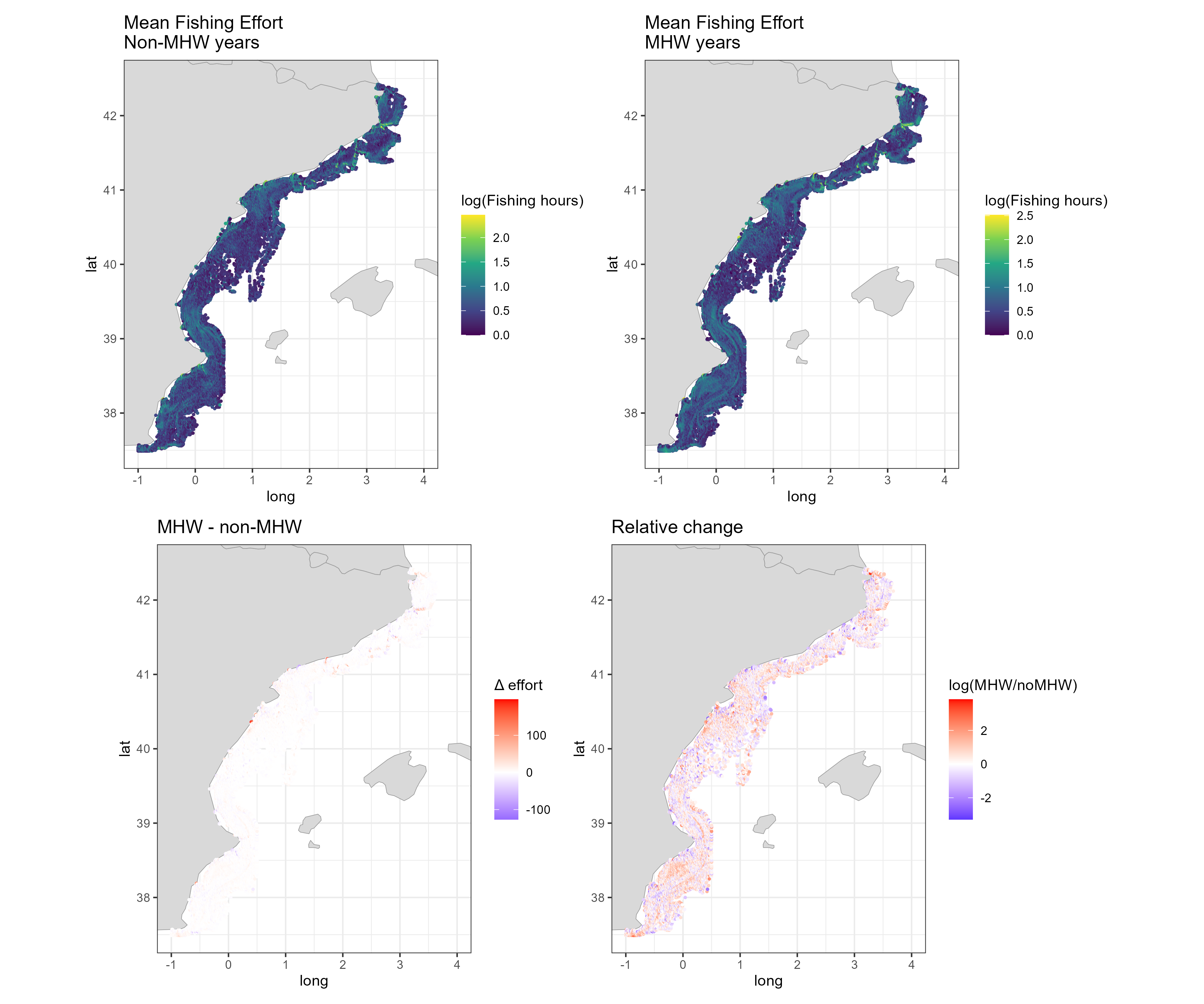
There is no consistent difference in fleet behaviour between strong and weak heatwave summers in either area. Total trawling hours differ by +1.9% in GSA 6 and -1.3% in the Adriatic, well within the spread between individual summers, and the number of vessels, the depth and distance to coast of fishing and the share of effort on the shelf barely change. The cell map shows a mosaic of local increases and decreases rather than a coherent shift. This contrasts with Section 3.2, where effort appeared higher in heatwave years: with the early, low-AIS years removed from the contrast, that difference disappears.
2c.11.1 Do strong and weak heatwave summers use the same fishing grounds?
Similar totals could hide a move to other grounds. Three spatial measures test this on the 0.05° grid, for each pair of summers:
Distribution overlap (Schoener’s D): D = 1 − ½ Σ |pᵢ − qᵢ|, where pᵢ and qᵢ are the shares of a summer’s trawling hours in cell i. D = 1 when effort is spread identically over the cells, 0 when the two summers share no cell.
Core grounds: for each summer, the smallest set of cells holding 80% of its trawling hours. Their overlap between two summers is measured with the Jaccard index (cells core in both / cells core in either).
Centre of gravity: the effort-weighted mean position of trawling in each summer.
If heatwaves move the fleet, overlap between a strong and a weak summer should be lower than between two summers of the same kind.
Pairwise overlap of trawling between summers
fleet_y <-read.csv("outputs/fleet_MHW_cells_year.csv")yr_class <-distinct(fleet_y, region, year, class)core_cells <-function(d, share =0.8) { d <-arrange(d, desc(hours)) d[cumsum(d$hours) /sum(d$hours) <= share |seq_len(nrow(d)) ==1, c("Lon", "Lat")]}pair_overlap <-function(reg) { d <-filter(fleet_y, region == reg) yrs <-sort(unique(d$year))bind_rows(lapply(combn(yrs, 2, simplify =FALSE), \(p) { a <-filter(d, year == p[1]); b <-filter(d, year == p[2]) m <-full_join(a |>transmute(Lon, Lat, pa = hours /sum(hours)), b |>transmute(Lon, Lat, pb = hours /sum(hours)), by =c("Lon", "Lat")) |>mutate(across(c(pa, pb), \(x) coalesce(x, 0))) ca <-core_cells(a); cb <-core_cells(b)tibble(region = reg, y1 = p[1], y2 = p[2],D =1-0.5*sum(abs(m$pa - m$pb)),jaccard =nrow(inner_join(ca, cb, by =c("Lon", "Lat"))) /nrow(distinct(bind_rows(ca, cb)))) }))}overlap_g <-bind_rows(lapply(unique(fleet_y$region), pair_overlap)) |>left_join(yr_class |>rename(y1 = year, c1 = class), by =c("region", "y1")) |>left_join(yr_class |>rename(y2 = year, c2 = class), by =c("region", "y2")) |>mutate(pair =case_when(c1 == c2 & c1 =="strong"~"Strong vs strong", c1 == c2 ~"Weak vs weak", TRUE~"Strong vs weak"))# Centre of gravity per summer and its distance to the area's six-summer centrecog_g <- fleet_y |>group_by(region, year, class) |>summarise(lon =weighted.mean(Lon, hours), lat =weighted.mean(Lat, hours), .groups ="drop") |>group_by(region) |>mutate(shift_km =sqrt(((lon -mean(lon)) *111.32*cos(mean(lat) * pi /180))^2+ ((lat -mean(lat)) *110.57)^2)) |>ungroup()
Show code
ov_long <-bind_rows(overlap_g, overlap_g |>rename(y1 = y2, y2 = y1, c1 = c2, c2 = c1)) |>pivot_longer(c(D, jaccard), names_to ="measure") |>mutate(measure =recode(measure, D ="Schoener's D", jaccard ="Core grounds (Jaccard)"),mixed = pair =="Strong vs weak")ov_plot <-function(reg) { d <-filter(ov_long, region == reg) strong <-sort(unique(d$y1[d$c1 =="strong"])) lv <-c(sort(unique(d$y1[d$c1 =="weak"])), strong) d <-mutate(d, y1 =factor(y1, lv), y2 =factor(y2, lv)) face <-ifelse(lv %in% strong, "bold", "plain")ggplot(d, aes(y1, y2, fill = value)) +geom_tile(colour ="white", linewidth =0.6) +geom_tile(data =filter(d, mixed), colour ="black", linewidth =0.4, fill =NA) +geom_text(aes(label =sprintf("%.2f", value)), size =2.8) +scale_fill_gradient(low ="white", high = pal_ocean[["surface"]], limits =c(0.4, 1), oob = squish, name =NULL) +facet_wrap(~measure) +labs(title = reg, x =NULL, y =NULL) +theme_ocean(9) +theme(axis.text.x =element_text(face = face), axis.text.y =element_text(face = face),panel.grid =element_blank(), legend.position ="none")}ov_plot("GSA 6") /ov_plot("GSAs 17-18")
Figure 32: Overlap of trawling between every pair of summers, by area. Left: Schoener’s D between effort distributions on the 0.05° grid (1 = identical). Right: Jaccard overlap of core grounds (cells holding 80% of each summer’s hours). Bold years are strong heatwave summers. Pairs of a strong and a weak summer are outlined in black.
Table 19: Mean overlap of trawling between summers, by type of pair. Area: GSA 6 or GSAs 17-18. Pair: two strong heatwave summers, two weak ones, or one of each. Pairs: number of pairs of summers. Schoener’s D: mean overlap of the effort distributions (1 = identical). Core grounds (Jaccard): mean overlap of the cells holding 80% of each summer’s hours. Centre-of-gravity shift (km), given in the strong vs weak row: distance between the mean centre of gravity of the strong summers and that of the weak summers.
Area
Pair
Pairs
Schoener’s D
Core grounds (Jaccard)
Centre-of-gravity shift (km)
GSA 6
Strong vs strong
3
0.71
0.54
GSA 6
Strong vs weak
9
0.72
0.55
1.4
GSA 6
Weak vs weak
3
0.70
0.52
GSAs 17-18
Strong vs strong
3
0.71
0.56
GSAs 17-18
Strong vs weak
9
0.72
0.58
3.9
GSAs 17-18
Weak vs weak
3
0.72
0.58
2c.11.2 Overlap with red mullet habitat and with the heat
The same yearly effort can be related to the two layers of Section 2c, cell by cell: the red mullet biomass predicted for that summer’s year, and that summer’s heatwave intensity (nearest prediction cell, for trawling within 5 km of the prediction grid: 78% of the hours in GSA 6, where much trawling is deeper than the grid, and 94% in the Adriatic).
Show code
# Heat map of the strong summers: mean cumulative intensity per 0.05° cell over the strong yearsstrong_heat <- mhw_g |>semi_join(yr_class |>filter(class =="strong"), by =c("region", YEAR ="year")) |>mutate(Lon =floor(X /0.05) *0.05+0.025, Lat =floor(Y /0.05) *0.05+0.025) |>group_by(region, Lon, Lat) |>summarise(heat =mean(mhw_cum_intensity, na.rm =TRUE), .groups ="drop") |>filter(is.finite(heat)) |>group_by(region) |>mutate(heat_area =mean(heat)) |>ungroup()hab_g <- fleet_y |>filter(on_grid) |>left_join(bind_rows(readRDS("data/group/pred_6.rds") |>mutate(region ="GSA 6"),readRDS("data/group/pred_1718.rds") |>mutate(region ="GSAs 17-18")) |>group_by(region, year) |>summarise(q75 =quantile(dens, 0.75), .groups ="drop"),by =c("region", "year")) |>mutate(Lon =round(Lon, 3), Lat =round(Lat, 3)) |>left_join(strong_heat |>mutate(Lon =round(Lon, 3), Lat =round(Lat, 3)), by =c("region", "Lon", "Lat")) |>group_by(region, year, class) |>summarise(hot_share =sum(hours[dens >= q75]) /sum(hours),mhw_ratio =sum((heat * hours)[!is.na(heat)]) /sum(hours[!is.na(heat)]) /first(na.omit(heat_area)),.groups ="drop")kable(hab_g |>group_by(Area = region, Summer =recode(class, strong ="Strong MHW", weak ="Weak MHW")) |>summarise(`Effort in red mullet hotspots`=percent(mean(hot_share), 1),`Heatwave exposure ratio`=sprintf("%.2f", mean(mhw_ratio)),.groups ="drop"))
Table 20: Overlap of trawling with red mullet and with heatwaves, by area and type of summer (mean of three summers; trawling within 5 km of the prediction grid). Area: GSA 6 or GSAs 17-18. Summer: strong or weak heatwave summer. Effort in red mullet hotspots: share of trawling hours in the cells with the highest predicted red mullet biomass that year (top 25% of grid cells). Heatwave exposure ratio: mean heatwave intensity of the strong summers (cumulative, per cell) weighted by each summer’s trawling hours, divided by its mean over all grid cells (above 1: trawling sits in the cells that get hotter in heatwave summers; below 1: in the cooler cells). The same heat map is used for both types of summer, so a lower ratio in strong summers than in weak ones would mean the fleet moves away from the heat.
Figure 33: Core trawling grounds (cells holding 80% of the mean summer hours) in strong and weak heatwave summers, on the 0.05° grid. Blue-grey: core in both; red: core only in strong heatwave summers; dark blue: core only in weak ones.
The fleets fish the same grounds in strong and weak heatwave summers. In GSA 6, the overlap between a strong and a weak summer (D = 0.72) is as high as between two summers of the same kind (0.71 and 0.7), and the same holds in the Adriatic (0.72 against 0.71 and 0.72). The centre of gravity of trawling moves by 1.4 km in GSA 6 and 3.9 km in the Adriatic between the two types of summer, and 72% and 73% of core cells are core in both. The cells that are core in only one type of summer are scattered along the edges of the main grounds, as expected from year-to-year variation. The share of effort on red mullet hotspots barely changes (13% against 14% in GSA 6, 23% against 20% in the Adriatic, strong against weak summers). Relative to where heatwaves strike, the fleet is not displaced either: the heatwave exposure ratio is 0.99 against 0.99 in GSA 6 and 1.06 against 1.05 in the Adriatic (strong against weak summers). Ratios close to 1 in both types of summer mean that trawling is spread across hot and cool cells in proportion to the grid, and does not shift away from the cells that heat up most.
Discussion points. (1) With three summers per group, year-to-year differences that have nothing to do with heatwaves (fuel prices, closures, COVID-19 in 2020, a strong heatwave summer in GSA 6 and a weak one in the Adriatic) weigh as much as the heatwave contrast. (2) Summer-level metrics may hide short-term responses: heatwaves last days to weeks. A stronger design uses the daily data already downloaded, comparing effort on heatwave days and on other days of the same summers in the same cells. (3) Across all summers from 2015 to 2021, a regression of each fleet metric on the area’s heatwave intensity would use all years instead of six. (4) Management measures that changed over the period, such as spatial closures, should be checked before reading local patches in the map as heatwave responses.
2c.12 Heatwaves and predicted red mullet biomass
The group’s preliminary report on the Adriatic (Mullus barbatus in GSA 6 and GSA 17–18 — preliminary report, with code shared on 22 October) asks whether heatwaves relate to red mullet biomass at two scales: across years, through the biomass index, and within years, through the year-specific part of the predictions (epsilon_st, the spatio-temporal field: how much a cell’s log biomass departs from its usual level in a given year). The analysis is reproduced here for the Adriatic and extended to GSA 6, with the heatwave metrics of Section 2c.10 and, as the report proposes as a next step, depth and latitude added to the within-year model.
Join predictions, trawling and heatwaves (same summer and previous summer)
rel_g <-bind_rows(lapply(c(`GSA 6`="6", `GSAs 17-18`="1718"), \(a) { mhw <-read.csv(file.path("outputs", paste0("MHW_grid_", a, ".csv"))) |>mutate(X =round(X, 4), Y =round(Y, 4)) |>arrange(X, Y, YEAR) |>group_by(X, Y) |>mutate(mhw_lag =lag(mhw_cum_intensity)) |>ungroup() |>select(X, Y, year = YEAR, mhw = mhw_cum_intensity, mhw_lag)readRDS(file.path("data/group", paste0("pred_", a, ".rds"))) |>mutate(X =round(X, 4), Y =round(Y, 4)) |>left_join(mhw, by =c("X", "Y", "year"))}), .id ="region")annual_g <- rel_g |>group_by(region, year) |>summarise(`Biomass index`=sum(dens * cell_km2) /1000, # tonnes`Trawling hours`=sum(trawl_y),`MHW, same summer`=mean(mhw, na.rm =TRUE),`MHW, previous summer`=mean(mhw_lag, na.rm =TRUE), .groups ="drop")
Figure 34: Annual series, 2014-2021, standardised within each area (z-scores): predicted red mullet biomass index, total trawling hours on the prediction grid, and mean summer cumulative heatwave intensity in the same and in the previous summer. Shaded: the three strongest heatwave summers of each area.
Table 21: Spearman rank correlations between the annual series, 2014-2021 (eight years), by area. Area: GSA 6 or GSAs 17-18. Biomass vs MHW (same summer), Biomass vs MHW (previous summer), Biomass vs trawling: correlation of the predicted biomass index with the mean summer cumulative heatwave intensity of the same summer, of the previous summer, and with total trawling hours. Strong MHW summers: the three strongest summers from 2014, with the change in the biomass index from the previous year.
Area
Biomass vs MHW (same summer)
Biomass vs MHW (previous summer)
Biomass vs trawling
Strong MHW summers
GSA 6
0.53
-0.12
0.21
2017 (-7%), 2018 (-3%), 2020 (+51%)
GSAs 17-18
-0.14
-0.29
0.26
2015 (-25%), 2018 (-47%), 2019 (+17%)
In the Adriatic, as the group’s report found, the biomass index falls in the two strongest heatwave summers, 2015 and 2018, and recovers the next year, but the overall correlation is weak because 2020, with almost no heatwave, has the lowest index. GSA 6 shows the opposite pattern: its strongest heatwave summers (2017, 2020) are among its highest-biomass years. With eight years per area and two areas behaving in opposite ways, the annual series do not support a general heatwave effect on red mullet biomass.
Within years
Within-year GAM of the spatio-temporal deviation (epsilon_st)
rel_gam <-lapply(split(rel_g, rel_g$region), \(d) { d <-filter(d, !is.na(mhw), !is.na(mhw_lag))gam(epsilon_st ~s(mhw, k =4) +s(mhw_lag, k =4) +s(log1p(trawl_y), k =4) +s(depth, k =4) +s(Y, k =4) +factor(year),data = d, method ="REML")})
Show code
term_df <-bind_rows(lapply(names(rel_gam), \(a) { m <- rel_gam[[a]]; d <- m$modelbind_rows(lapply(c(mhw ="MHW, same summer (°C days)", mhw_lag ="MHW, previous summer (°C days)",trawl ="Trawling hours (log1p)"), \(lab) { v <-names(which(c(mhw ="MHW, same summer (°C days)", mhw_lag ="MHW, previous summer (°C days)",trawl ="Trawling hours (log1p)") == lab)) xs <-if (v =="trawl") log1p(d$`log1p(trawl_y)`|>expm1()) else d[[v]] grid <-seq(quantile(xs, 0.01), quantile(xs, 0.99), length.out =100) nd <- d[rep(1, 100), ]for (cc inc("mhw", "mhw_lag", "depth", "Y")) nd[[cc]] <-median(d[[cc]]) nd$trawl_y <-median(expm1(d$`log1p(trawl_y)`))if (v =="trawl") nd$trawl_y <-expm1(grid) else nd[[v]] <- grid tm <-predict(m, newdata = nd, type ="terms", se.fit =TRUE) col <-switch(v, mhw ="s(mhw)", mhw_lag ="s(mhw_lag)", trawl ="s(log1p(trawl_y))")tibble(region = a, term = lab, x = grid, fit = tm$fit[, col], se = tm$se.fit[, col]) }))}))term_df <-mutate(term_df, term =factor(term, c("MHW, same summer (°C days)", "MHW, previous summer (°C days)", "Trawling hours (log1p)")))ggplot(term_df, aes(x, fit, colour = region, fill = region)) +geom_hline(yintercept =0, colour ="grey70") +geom_ribbon(aes(ymin = fit -1.96* se, ymax = fit +1.96* se), alpha =0.2, colour =NA) +geom_line(linewidth =0.9) +scale_colour_manual(values = grp_cols, name =NULL) +scale_fill_manual(values = grp_cols, name =NULL) +facet_grid(region ~ term, scales ="free_x") +labs(x =NULL, y ="Partial effect on epsilon_st (log scale)") +theme_ocean()
Figure 35: Within-year relationships between the spatio-temporal deviation of predicted red mullet log biomass (epsilon_st) and heatwave intensity in the same summer, heatwave intensity in the previous summer, and trawling hours (log scale), from a GAM that also includes depth, latitude and a year factor. Lines: partial effects; bands: approximate 95% intervals; rugs: data. The year factor removes the annual means, so the curves describe contrasts between cells within the same year.
Within years, the relationships are small in GSA 6 and not monotonic in the Adriatic. There, with depth and latitude in the model, biomass is slightly below its usual level in cells with moderate heatwave exposure (around 30 °C days) and above it in the most exposed cells, as in the group’s report; cells that were hot in the previous summer tend to have slightly lower biomass. Trawling effort shows no relationship in either area. None of this reproduces the annual dips of 2015 and 2018, consistent with the group’s reading that, if heatwaves matter in the Adriatic, they act on the availability of red mullet to the summer survey across the whole area rather than through local losses. Curves are shown over the central 98% of the data.
Discussion points. (1) As the group’s report notes, epsilon_st is a smoothed model output and cells are spatially dependent, so the GAM’s p-values are not meaningful and are not shown. (2) A direct test is to add heatwave intensity, or a bottom temperature anomaly, as a covariate of the sdmTMB model fitted to the hauls. (3) Heatwaves are defined from sea surface temperature; red mullet lives on the bottom, where, especially in the stratified central Adriatic in summer, conditions can differ.
3. Marine heatwaves and fleet behaviour
3.1 Detecting marine heatwaves
Marine heatwaves (MHWs) are periods of at least five consecutive days during which SST exceeds the seasonally varying 90th percentile of a baseline climatology (Hobday et al. 2016). They are detected with heatwaveR on daily L4 SST (Copernicus SST_MED_SST_L4_REP_OBSERVATIONS_010_021), extracted at each prediction grid point in GSA 6. Only events peaking in June-August are kept, when thermal stress is highest in the Mediterranean.
Detect MHWs at each grid point (not evaluated: daily SST NetCDF)
Table 22: Summer marine heatwave (MHW) metrics by year, averaged over the GSA 6 grid points (events peaking in June-August). Year. Events: mean number of MHW events per grid point. MHW days: mean number of days under MHW conditions. Mean intensity (°C): mean SST anomaly during events, relative to the seasonal climatology. Cumulative intensity (°C days): sum of the daily anomalies over all events. Used as: role of the year in the fleet comparison (MHW, non-MHW or not used).
Year
Events
MHW days
Mean intensity (°C)
Cumulative intensity (°C days)
Used as
2012
0.42
2.8
0.63
4.3
not used
2013
0.09
0.6
0.18
1.2
non-MHW
2014
0.00
0.0
0.00
0.0
non-MHW
2015
1.06
11.5
1.24
19.0
not used
2016
0.00
0.0
0.00
0.0
non-MHW
2017
1.58
19.6
2.39
46.6
MHW
2018
1.34
13.9
1.81
27.4
MHW
2019
0.58
4.0
0.84
8.3
not used
2020
1.78
15.8
1.55
28.4
MHW
2021
0.30
1.9
0.67
4.5
not used
Show code
ggplot(mhw.gsa, aes(YEAR, mhw_cum_intensity, fill = group)) +geom_col() +scale_fill_manual(values =c("MHW"= pal_ocean[["alert"]],"non-MHW"= pal_ocean[["surface"]],"not used"= pal_ocean[["grey"]]), name =NULL) +scale_x_continuous(breaks =2012:2021) +labs(x =NULL, y ="Cumulative intensity (°C days)") +theme_ocean()
Figure 36: Mean summer cumulative MHW intensity across GSA 6 grid cells, coloured by how each year is used in the fleet comparison.
Figure 37: Summer cumulative MHW intensity per grid cell, 2012-2021.
Cumulative intensity combines duration and magnitude into a single measure of thermal stress. Summers 2017, 2018 and 2020 stand out, with 2015 also strong. 2014 and 2016 had no summer events.
Discussion point: baseline length. The climatology is built on 2010-2021, against the 30-year baseline recommended by Hobday et al. (2016). A short, recent baseline that already contains the warming trend raises the threshold and under-detects events.
3.2 Trawling in heatwave and non-heatwave summers
Daily trawler effort at 0.01° is pulled for June-August of the six selected years, clipped to the GSA 6 polygon. Each cell is given a depth (NOAA ETOPO via marmap) and a distance to the nearest coastline (Natural Earth), and fleet indicators are compared between the two groups of years.
Table 23: Summer trawler effort in GSA 6 in MHW years (2017, 2018, 2020) and non-MHW years (2013, 2014, 2016), from daily GFW AIS apparent fishing hours on a 0.01° grid. Period: MHW or non-MHW years. Cells fished: number of 0.01° cells with trawler effort in at least one year of the period. Total mean hours: sum over cells of the mean annual summer fishing hours. Median hours per cell: median of the per-cell mean annual summer fishing hours.
Period
Cells fished
Total mean hours
Median hours per cell
MHW years
26704
133802
2.93
non-MHW years
26052
113376
2.42
Of the cells fished in at least one period, 21,911 were fished in both and enter the change maps. In 56% of them, effort was higher in heatwave summers.
Discussion point: confounding with AIS uptake. The non-MHW years include 2013 and 2014, when trawler AIS coverage was still growing (Step 1). Higher effort in MHW years is therefore expected even with no change in behaviour. Picking contrasting years from 2015 onward (e.g. 2016 vs 2017), or comparing effort per vessel, would separate the two. Two smaller points: cells missing in a year are not counted as zero in fishing.maps, which inflates means, and depth and distance to coast are averaged over cells rather than weighted by fishing hours.
4. Climate-fisheries vulnerability index
Vulnerability is classically framed as exposure plus sensitivity minus adaptive capacity. The Climate-Fisheries Vulnerability Index (CFVI) combines three indicators, each rescaled to 0-1 and averaged with equal weights:
Exposure: summer cumulative MHW intensity in 2021.
Sensitivity: percentage change in predicted fish abundance 2012-2021, on the abundance scale (the sign is flipped so that habitat loss raises vulnerability).
Table 24: Distribution of the climate-fisheries vulnerability index (CFVI) components across GSA 6 grid cells. component: exposure (2021 cumulative MHW intensity), sensitivity (decline in predicted total fish abundance, 2012-2021), pressure (2021 trawler fishing hours) and CFVI (the mean of the three), each min-max scaled to 0-1. median: median score across cells. share zero: share of cells scoring exactly 0.
component
median
share zero
exposure
0.00
71%
sensitivity
0.80
0%
pressure
0.08
8%
CFVI
0.33
0%
The highest index values sit off the northern Catalan coast (Cap de Creus to Roses) and in nearshore cells off the Ebro delta and Valencia, where moderate heatwave exposure overlaps with heavy trawling and predicted abundance loss.
Discussion point: time windows and scaling. Exposure uses a single, mild heatwave year: 71% of cells score exactly 0, so the index is mostly driven by pressure and sensitivity in the rest of GSA 6. Pressure is very skewed and min-max scaling squashes most cells near 0. Sensitivity includes the extrapolated coastal cells of Step 2. More defensible choices: mean exposure over 2015-2021, log-transformed effort, habitat change from within the sampled range only, and a check of how the hotspots move under different weights.
Summary and next steps
The pipeline links survey, environmental, heatwave and AIS data into a coherent spatial workflow. Before interpreting the results, four points are worth addressing as a group:
AIS ramp-up: start comparisons in 2015, or normalise effort per vessel, so that changes in AIS coverage are not read as changes in fishing.
Extrapolation: predict in the survey months (May-June) and within the sampled depth range, so that habitat change and the sensitivity score are not driven by out-of-range coastal cells.
Zeros: treat unmatched hauls and unfished cells consistently as zero effort in fitting, prediction and averaging.
Index design: align the time windows of the three CFVI components and test sensitivity to transformation and weights.
For red mullet, the group’s spatio-temporal model (Section 2c) extends the analysis to the Adriatic and gives a broadly stable GSA 6 biomass index from 2015 to 2021; like the Tweedie GAM of Section 2b, it shows no increase. In Section 2b, the model with zeros, a Tweedie family and depth explains about half the deviance and predicts a widespread decline in June density from 2015 to 2021 that holds when fishing effort is held constant. Natural next steps are to identify which environmental term drives the decline, check it against the observed MEDITS trend, and feed the red mullet habitat change into the vulnerability index in place of total fish abundance.
Smaller fixes (grid alignment in the haul join, MHW baseline length, weighted depth and distance means, the unfinished daily block in Script 1) are listed in review_notes.md.